Direction Stopped Mattering: Code and Graph in One Loop

TL;DR. Flowfile has two front doors that build the same flow: the visual canvas and a Polars-shaped Python API called FlowFrame. Both edit the same graph, and a flow can be exported as a standalone Polars script you’d actually write. (A SQL editor sits alongside as a query and visualization surface over the catalog — same data, different job.) The interesting story isn’t any one feature — it’s that the direction someone starts from stopped mattering.

The two-camp problem

Most data tools pick a camp. Visual tools (Alteryx, classic SSIS, Talend) make the canvas the centre of the universe; the code is something the tool talks to internally and reluctantly exposes for export. Code-first tools (dbt, Polars, Spark scripts) make text the centre; the visual layer, if there is one, is a read-only DAG render that explodes as soon as you try to edit it.

Both work. Both also make people choose. The analyst who thinks visually has to convince the engineering team to host their Alteryx licence. The engineer who lives in code has to forgo the at-a-glance lineage view that a canvas gives for free.

The split usually looks like a tooling problem. It’s a layer problem. If the canvas and the code don’t share a representation, they can never round-trip without something getting lost. Flowfile’s bet is that a single Pydantic-modelled graph, edited from both sides, removes the choice.

One graph, two editors

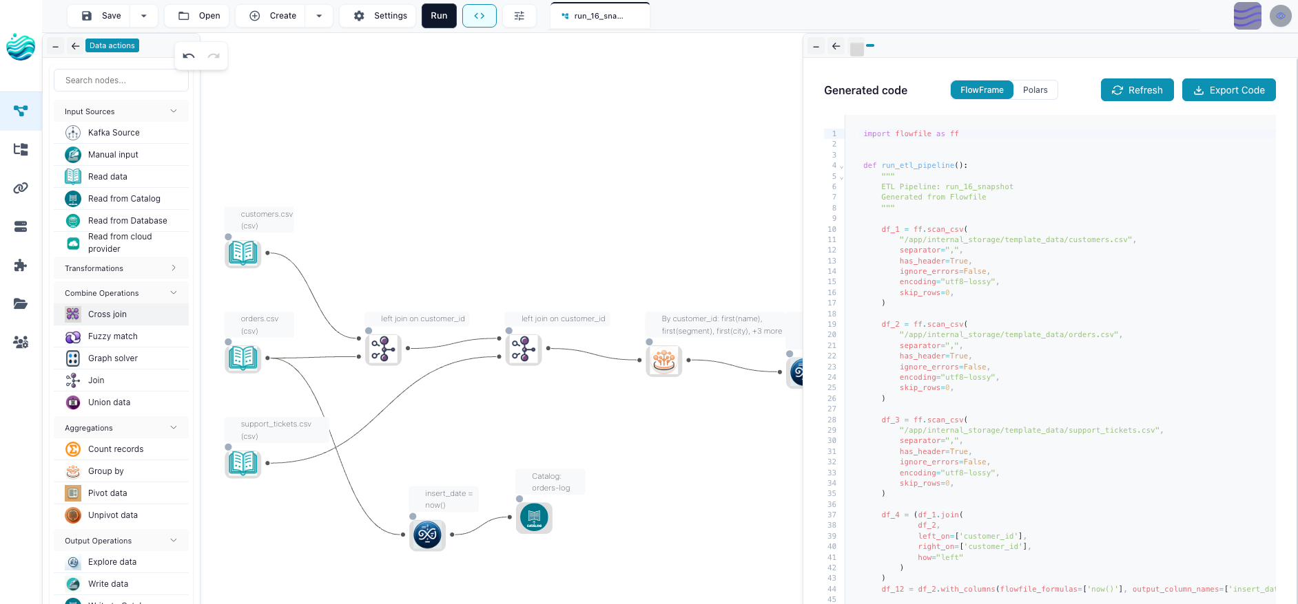
Underneath every Flowfile flow is a flow_graph object — a DAG of typed Pydantic settings, one per node. The graph is the only thing that gets serialised to disk (as YAML). Everything else is a way of editing it.

The canvas is a Vue 3 + VueFlow editor. Drop a node, fill in a form, the form is a binding to the same Pydantic model the API would mutate by hand. There’s no second representation.

FlowFrame, the Python API, mirrors Polars. Each method call adds a node:

import flowfile_frame as ff

orders = ff.read_parquet("data/orders.parquet")
top_customers = (
    orders
    .filter(ff.col("status") == "paid")
    .group_by("customer_id")
    .agg(ff.col("amount").sum().alias("revenue"))
    .sort("revenue", descending=True)
    .head(100)
)

top_customers.save_graph("flows/top_customers.yaml")

That’s it. The graph is constructed as the methods run. top_customers.to_graph() returns the same flow_graph the canvas would have produced for an equivalent set of clicks. Open the saved YAML in the desktop app and the canvas shows up — Read Parquet → Filter → Group By → Sort → Head — with all the wiring and column metadata already there.

Same graph. Two editors. Neither is privileged.

The SQL editor lives next door

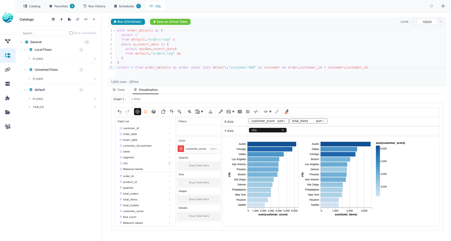
Flowfile’s SQL editor isn’t a third editor of the same graph — it’s an exploration surface over the catalog, and the distinction is worth being explicit about.

The editor runs queries against every catalog table through a Polars SQLContext. Results stream into Graphic Walker, where you drag fields onto axes and switch chart types interactively. Save as Visualization stores the Graphic Walker workspace — chart spec plus the inline SQL — and re-runs the query each time the visualization is opened. The data is never embedded; the chart always reflects the current state of the catalog tables it queries.

What the editor doesn’t do is produce a flow. There is no Save as Flow button, no synthesis of catalog_reader → sql_query nodes onto the canvas, no schedule that fires when a saved query updates. SQL queries and the visualizations built on top of them are persisted as their own catalog artifact, separate from the flow graph.

That’s a deliberate trade. The canvas and FlowFrame edit pipelines — batched, scheduled, exportable as code. The SQL editor explores data — ad-hoc queries, visual analysis, charts that stay live as the underlying tables update. Both surfaces share the same catalog underneath, but they’re solving different jobs and the design admits that instead of pretending otherwise.

The export that closes the loop

A graph that only the source tool can read is a trap. Flowfile’s escape hatch is export_flow_to_polars(flow) — walk the graph, ask each node to render its Polars equivalent, emit a standalone script. The output looks like this:

# Generated by Flowfile
import polars as pl

orders = pl.scan_parquet("data/orders.parquet")
top_customers = (
    orders
    .filter(pl.col("status") == "paid")
    .group_by("customer_id")
    .agg(pl.col("amount").sum().alias("revenue"))
    .sort("revenue", descending=True)
    .head(100)
    .collect()
)

No Flowfile import. No runtime dependency. If the laptop with the canvas vanishes, the script still runs anywhere Polars runs. There’s a sister exporter, export_flow_to_flowframe(flow), that emits FlowFrame code instead — useful when you want the export to round-trip back into the canvas without losing visual information.

The export isn’t a separate translation step. The Polars rendering is the same code the engine runs internally to execute the node, with placeholders for the inputs swapped to script variables. There’s no second implementation that can drift.

What the round-trip is actually for

The point of all this isn’t that you’d convert in every direction every day. It’s that the conversion existing changes how you treat the artifact.

A flow becomes a Polars script you can hand to a colleague who lives in code — here’s what this canvas does in the language you read all day. A Polars script becomes something you can paste into the canvas as a starting frame and refine visually — by writing the FlowFrame version and saving the graph. The same idea, in two notations, reduced to one underlying object that the rest of Flowfile (catalog, scheduler, lineage) can act on.

This matters most for the part of the team that doesn’t usually get included in tooling decisions. The analyst who can follow a visual flow but not a 200-line Polars script can now look at the same artifact as the engineer who wrote it. The engineer can pull the canvas up to argue about a join condition the way you’d point at a diagram. Nobody has to context-switch into a different language to discuss the same logic.

Where this actually breaks

The honest paragraph. Three places it isn’t seamless yet.

Custom Python nodes don’t export to plain Polars. A node whose body imports scikit-learn or hits an internal API can’t be written as pl.col(...). The Polars exporter raises UnsupportedNodeError in that case. The FlowFrame exporter handles it by emitting the user’s code inside a @flow_function-style wrapper, but the result needs FlowFrame to run. If you want Flowfile-free Polars and you’re using script nodes, you’ll have to inline them by hand.

Plain Polars code doesn’t reverse-engineer into a canvas. There’s no AST parser sitting behind a Paste your script here box. The way you go from a Polars script to a graph is by rewriting it in FlowFrame, which is mechanical (the methods are the same) but not free. If anyone tells you otherwise about a tool, ask to see the conversion of pl.col("x").map_elements(lambda x: ...).

SQL on the canvas is more constrained than Polars expressions. The canvas SQL node runs through Polars SQLContext, which covers most analytics SQL but not every dialect feature. A query that uses Postgres window-frame syntax or recursive CTEs won’t translate cleanly. You’d write that as a database_reader node that hits the actual database instead.

These aren’t theoretical limits. They’re the shape of where the model breaks, and saying so up front is more useful than pretending the round-trip is universal.

Why one graph beats two integrations

The alternative — two tools that integrate — looks like this in practice: the canvas exports to YAML, a converter rewrites it as a dbt model or a Python script, and the two halves drift. Each step has its own version skew, its own list of unsupported nodes, its own bug tracker. Every team I’ve watched try this ends up with one canonical layer (usually the code) and a read-only view of it that gradually goes out of date.

A single graph with two editors avoids the integration problem by not having an integration. The canvas and FlowFrame aren’t talking to each other. They’re each talking to the same Pydantic models in the same process. When the data model changes, both change at once because there’s nothing to coordinate.

That’s the real claim. Not Flowfile is more powerful. Flowfile is the same as if you took your existing pipeline tool and stopped letting the layers be different products.

Where to start

If the visual side is your home, open the desktop app and click Export on any flow — the script that comes out is what your decisions look like in code. If code is your home, pip install flowfile_frame, build a flow with the FlowFrame API, and save_graph(...) it to YAML — open the YAML in the app and the canvas is just there. If you mostly query the catalog from SQL, register a couple of tables, open the SQL editor, and save the visualization that comes out — different door, different job, same data underneath.

Direction stopped mattering. The graph is the unit of work; the rest is taste.

---

Related reads: Catalogs Make Data Easy. Open Formats Keep It Yours. for the catalog tables the SQL editor queries, Your Lineage Graph Should Run Your Pipelines for what those graphs do once they exist, and Polars vs Pandas in 2026 for why the underlying engine matters.